install.packages("psych")
install.packages("corrplot")
install.packages("ggplot2")
install.packages("caret")
install.packages("ggpubr")
install.packages("klaR")32 Naive-Bayes ile Meme Kanser Veri Analizi
İlk olarak aşağıda bulunan paketleri kurmanız gerekidir:
Daha sonra bu paketleri yükleyelim:
corrplot 0.95 loaded
Attaching package: 'ggplot2'The following objects are masked from 'package:psych':
%+%, alphaLoading required package: latticeLoading required package: MASSBu çalışmada kullanılan tutorial:
https://www.kaggle.com/code/lbronchal/breast-cancer-dataset-analysis
Veri setimizi alalım (Siz buraya kendi dosya yolunuzu yazacaksınız). Veri seti link: https://www.kaggle.com/code/lbronchal/breast-cancer-dataset-analysis/input
İlk olarak verimizi yükleyelim:
bc_data <- read.csv("https://raw.githubusercontent.com/emrahkirdok/ybva/main/05-istatistik/data.csv")Teşhisi faktör olarak düzenleyelim (M:malign tümör, B:benign tümör) ve veri setini inceleyelim:
       id            diagnosis  radius_mean      texture_mean
 Min.   :     8670   B:357     Min.   : 6.981   Min.   : 9.71
 1st Qu.:   869218   M:212     1st Qu.:11.700   1st Qu.:16.17
 Median :   906024             Median :13.370   Median :18.84
 Mean   : 30371831             Mean   :14.127   Mean   :19.29
 3rd Qu.:  8813129             3rd Qu.:15.780   3rd Qu.:21.80
 Max.   :911320502             Max.   :28.110   Max.   :39.28
 perimeter_mean     area_mean      smoothness_mean   compactness_mean
 Min.   : 43.79   Min.   : 143.5   Min.   :0.05263   Min.   :0.01938
 1st Qu.: 75.17   1st Qu.: 420.3   1st Qu.:0.08637   1st Qu.:0.06492
 Median : 86.24   Median : 551.1   Median :0.09587   Median :0.09263
 Mean   : 91.97   Mean   : 654.9   Mean   :0.09636   Mean   :0.10434
 3rd Qu.:104.10   3rd Qu.: 782.7   3rd Qu.:0.10530   3rd Qu.:0.13040
 Max.   :188.50   Max.   :2501.0   Max.   :0.16340   Max.   :0.34540
 concavity_mean    concave.points_mean symmetry_mean    fractal_dimension_mean
 Min.   :0.00000   Min.   :0.00000     Min.   :0.1060   Min.   :0.04996
 1st Qu.:0.02956   1st Qu.:0.02031     1st Qu.:0.1619   1st Qu.:0.05770
 Median :0.06154   Median :0.03350     Median :0.1792   Median :0.06154
 Mean   :0.08880   Mean   :0.04892     Mean   :0.1812   Mean   :0.06280
 3rd Qu.:0.13070   3rd Qu.:0.07400     3rd Qu.:0.1957   3rd Qu.:0.06612
 Max.   :0.42680   Max.   :0.20120     Max.   :0.3040   Max.   :0.09744
   radius_se        texture_se      perimeter_se       area_se
 Min.   :0.1115   Min.   :0.3602   Min.   : 0.757   Min.   :  6.802
 1st Qu.:0.2324   1st Qu.:0.8339   1st Qu.: 1.606   1st Qu.: 17.850
 Median :0.3242   Median :1.1080   Median : 2.287   Median : 24.530
 Mean   :0.4052   Mean   :1.2169   Mean   : 2.866   Mean   : 40.337
 3rd Qu.:0.4789   3rd Qu.:1.4740   3rd Qu.: 3.357   3rd Qu.: 45.190
 Max.   :2.8730   Max.   :4.8850   Max.   :21.980   Max.   :542.200
 smoothness_se      compactness_se      concavity_se     concave.points_se
 Min.   :0.001713   Min.   :0.002252   Min.   :0.00000   Min.   :0.000000
 1st Qu.:0.005169   1st Qu.:0.013080   1st Qu.:0.01509   1st Qu.:0.007638
 Median :0.006380   Median :0.020450   Median :0.02589   Median :0.010930
 Mean   :0.007041   Mean   :0.025478   Mean   :0.03189   Mean   :0.011796
 3rd Qu.:0.008146   3rd Qu.:0.032450   3rd Qu.:0.04205   3rd Qu.:0.014710
 Max.   :0.031130   Max.   :0.135400   Max.   :0.39600   Max.   :0.052790
  symmetry_se       fractal_dimension_se  radius_worst   texture_worst
 Min.   :0.007882   Min.   :0.0008948    Min.   : 7.93   Min.   :12.02
 1st Qu.:0.015160   1st Qu.:0.0022480    1st Qu.:13.01   1st Qu.:21.08
 Median :0.018730   Median :0.0031870    Median :14.97   Median :25.41
 Mean   :0.020542   Mean   :0.0037949    Mean   :16.27   Mean   :25.68
 3rd Qu.:0.023480   3rd Qu.:0.0045580    3rd Qu.:18.79   3rd Qu.:29.72
 Max.   :0.078950   Max.   :0.0298400    Max.   :36.04   Max.   :49.54
 perimeter_worst    area_worst     smoothness_worst  compactness_worst
 Min.   : 50.41   Min.   : 185.2   Min.   :0.07117   Min.   :0.02729
 1st Qu.: 84.11   1st Qu.: 515.3   1st Qu.:0.11660   1st Qu.:0.14720
 Median : 97.66   Median : 686.5   Median :0.13130   Median :0.21190
 Mean   :107.26   Mean   : 880.6   Mean   :0.13237   Mean   :0.25427
 3rd Qu.:125.40   3rd Qu.:1084.0   3rd Qu.:0.14600   3rd Qu.:0.33910
 Max.   :251.20   Max.   :4254.0   Max.   :0.22260   Max.   :1.05800
 concavity_worst  concave.points_worst symmetry_worst   fractal_dimension_worst
 Min.   :0.0000   Min.   :0.00000      Min.   :0.1565   Min.   :0.05504
 1st Qu.:0.1145   1st Qu.:0.06493      1st Qu.:0.2504   1st Qu.:0.07146
 Median :0.2267   Median :0.09993      Median :0.2822   Median :0.08004
 Mean   :0.2722   Mean   :0.11461      Mean   :0.2901   Mean   :0.08395
 3rd Qu.:0.3829   3rd Qu.:0.16140      3rd Qu.:0.3179   3rd Qu.:0.09208
 Max.   :1.2520   Max.   :0.29100      Max.   :0.6638   Max.   :0.20750
Teşhis bilgisine bakalım:
prop.table(table(bc_data$diagnosis))
        B         M
0.6274165 0.3725835
Veri setini inceleyelim:
describe(bc_data) vars n mean sd median trimmed
id 1 569 30371831.43 125020585.61 906024.00 7344332.77
diagnosis* 2 569 1.37 0.48 1.00 1.34
radius_mean 3 569 14.13 3.52 13.37 13.82
texture_mean 4 569 19.29 4.30 18.84 19.04
perimeter_mean 5 569 91.97 24.30 86.24 89.74
area_mean 6 569 654.89 351.91 551.10 606.13
smoothness_mean 7 569 0.10 0.01 0.10 0.10
compactness_mean 8 569 0.10 0.05 0.09 0.10
concavity_mean 9 569 0.09 0.08 0.06 0.08
concave.points_mean 10 569 0.05 0.04 0.03 0.04
symmetry_mean 11 569 0.18 0.03 0.18 0.18
fractal_dimension_mean 12 569 0.06 0.01 0.06 0.06
radius_se 13 569 0.41 0.28 0.32 0.36
texture_se 14 569 1.22 0.55 1.11 1.16
perimeter_se 15 569 2.87 2.02 2.29 2.51
area_se 16 569 40.34 45.49 24.53 31.69
smoothness_se 17 569 0.01 0.00 0.01 0.01
compactness_se 18 569 0.03 0.02 0.02 0.02
concavity_se 19 569 0.03 0.03 0.03 0.03
concave.points_se 20 569 0.01 0.01 0.01 0.01
symmetry_se 21 569 0.02 0.01 0.02 0.02
fractal_dimension_se 22 569 0.00 0.00 0.00 0.00
radius_worst 23 569 16.27 4.83 14.97 15.73
texture_worst 24 569 25.68 6.15 25.41 25.39
perimeter_worst 25 569 107.26 33.60 97.66 103.42
area_worst 26 569 880.58 569.36 686.50 788.02
smoothness_worst 27 569 0.13 0.02 0.13 0.13
compactness_worst 28 569 0.25 0.16 0.21 0.23
concavity_worst 29 569 0.27 0.21 0.23 0.25
concave.points_worst 30 569 0.11 0.07 0.10 0.11
symmetry_worst 31 569 0.29 0.06 0.28 0.28
fractal_dimension_worst 32 569 0.08 0.02 0.08 0.08
mad min max range skew
id 65567.98 8670.00 911320502.00 911311832.00 6.44
diagnosis* 0.00 1.00 2.00 1.00 0.53
radius_mean 2.82 6.98 28.11 21.13 0.94
texture_mean 4.17 9.71 39.28 29.57 0.65
perimeter_mean 18.84 43.79 188.50 144.71 0.99
area_mean 227.28 143.50 2501.00 2357.50 1.64
smoothness_mean 0.01 0.05 0.16 0.11 0.45
compactness_mean 0.05 0.02 0.35 0.33 1.18
concavity_mean 0.06 0.00 0.43 0.43 1.39
concave.points_mean 0.03 0.00 0.20 0.20 1.17
symmetry_mean 0.03 0.11 0.30 0.20 0.72
fractal_dimension_mean 0.01 0.05 0.10 0.05 1.30
radius_se 0.16 0.11 2.87 2.76 3.07
texture_se 0.47 0.36 4.88 4.52 1.64
perimeter_se 1.14 0.76 21.98 21.22 3.43
area_se 13.63 6.80 542.20 535.40 5.42
smoothness_se 0.00 0.00 0.03 0.03 2.30
compactness_se 0.01 0.00 0.14 0.13 1.89
concavity_se 0.02 0.00 0.40 0.40 5.08
concave.points_se 0.01 0.00 0.05 0.05 1.44
symmetry_se 0.01 0.01 0.08 0.07 2.18
fractal_dimension_se 0.00 0.00 0.03 0.03 3.90
radius_worst 3.65 7.93 36.04 28.11 1.10
texture_worst 6.42 12.02 49.54 37.52 0.50
perimeter_worst 25.01 50.41 251.20 200.79 1.12
area_worst 319.65 185.20 4254.00 4068.80 1.85
smoothness_worst 0.02 0.07 0.22 0.15 0.41
compactness_worst 0.13 0.03 1.06 1.03 1.47
concavity_worst 0.20 0.00 1.25 1.25 1.14
concave.points_worst 0.07 0.00 0.29 0.29 0.49
symmetry_worst 0.05 0.16 0.66 0.51 1.43
fractal_dimension_worst 0.01 0.06 0.21 0.15 1.65
kurtosis se
id 41.66 5241135.60
diagnosis* -1.73 0.02
radius_mean 0.81 0.15
texture_mean 0.73 0.18
perimeter_mean 0.94 1.02
area_mean 3.59 14.75
smoothness_mean 0.82 0.00
compactness_mean 1.61 0.00
concavity_mean 1.95 0.00
concave.points_mean 1.03 0.00
symmetry_mean 1.25 0.00
fractal_dimension_mean 2.95 0.00
radius_se 17.45 0.01
texture_se 5.26 0.02
perimeter_se 21.12 0.08
area_se 48.59 1.91
smoothness_se 10.32 0.00
compactness_se 5.02 0.00
concavity_se 48.24 0.00
concave.points_se 5.04 0.00
symmetry_se 7.78 0.00
fractal_dimension_se 25.94 0.00
radius_worst 0.91 0.20
texture_worst 0.20 0.26
perimeter_worst 1.04 1.41
area_worst 4.32 23.87
smoothness_worst 0.49 0.00
compactness_worst 2.98 0.01
concavity_worst 1.57 0.01
concave.points_worst -0.55 0.00
symmetry_worst 4.37 0.00
fractal_dimension_worst 5.16 0.00Korelasyon matrixi ile ilişkili olan verileri inceleyelim:
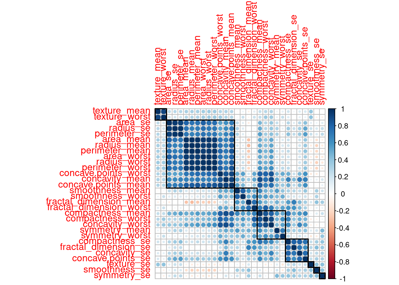
Etkenlerden birini seçip plotlayalım:
ggplot(bc_data, aes(x=texture_mean)) + geom_density(alpha=0.5, aes(fill=diagnosis)) + labs(title="Texture distribution by outcome")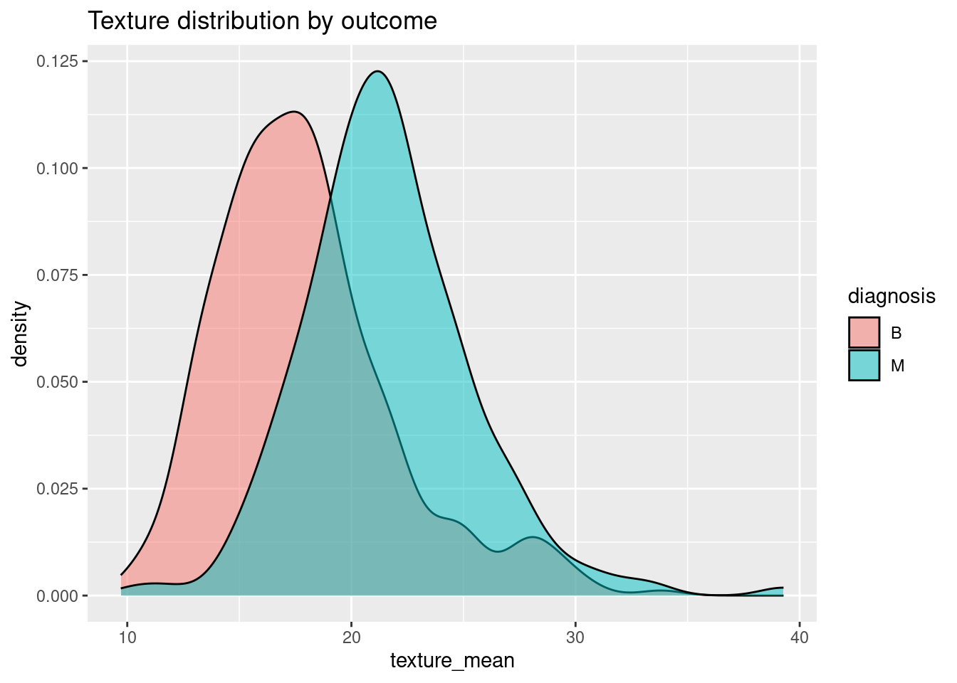
Şimdi yavaşça işin makine öğrenmesi kısmına başlıyoruz. Burada veri setimiz rastgele olarak iki parçaya bölünüyor: Makineye “öğreten” training set ve bunu test eden testing set.
set.seed(1234)
data_index <- createDataPartition(bc_data$diagnosis, p=0.7, list = FALSE)
train_data <- bc_data[data_index, -1]
test_data <- bc_data[-data_index, -1]
şimdi de bu bölünen kısımların oranlarına bakalım:
Veri setimiz:
prop.table(table(bc_data$diagnosis)) * 100
       B        M
62.74165 37.25835
Training setimiz:
prop.table(table(train_data$diagnosis)) * 100
       B        M
62.65664 37.34336
Testing setimiz:
prop.table(table(test_data$diagnosis)) * 100
       B        M
62.94118 37.05882
Verilerimizi görselleştirelim:
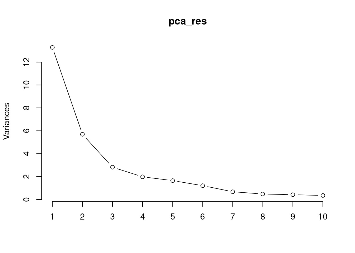
summary(pca_res)Importance of components:
PC1 PC2 PC3 PC4 PC5 PC6 PC7
Standard deviation 3.6444 2.3857 1.67867 1.40735 1.28403 1.09880 0.82172
Proportion of Variance 0.4427 0.1897 0.09393 0.06602 0.05496 0.04025 0.02251
Cumulative Proportion 0.4427 0.6324 0.72636 0.79239 0.84734 0.88759 0.91010
PC8 PC9 PC10 PC11 PC12 PC13 PC14
Standard deviation 0.69037 0.6457 0.59219 0.5421 0.51104 0.49128 0.39624
Proportion of Variance 0.01589 0.0139 0.01169 0.0098 0.00871 0.00805 0.00523
Cumulative Proportion 0.92598 0.9399 0.95157 0.9614 0.97007 0.97812 0.98335
PC15 PC16 PC17 PC18 PC19 PC20 PC21
Standard deviation 0.30681 0.28260 0.24372 0.22939 0.22244 0.17652 0.1731
Proportion of Variance 0.00314 0.00266 0.00198 0.00175 0.00165 0.00104 0.0010
Cumulative Proportion 0.98649 0.98915 0.99113 0.99288 0.99453 0.99557 0.9966
PC22 PC23 PC24 PC25 PC26 PC27 PC28
Standard deviation 0.16565 0.15602 0.1344 0.12442 0.09043 0.08307 0.03987
Proportion of Variance 0.00091 0.00081 0.0006 0.00052 0.00027 0.00023 0.00005
Cumulative Proportion 0.99749 0.99830 0.9989 0.99942 0.99969 0.99992 0.99997
PC29 PC30
Standard deviation 0.02736 0.01153
Proportion of Variance 0.00002 0.00000
Cumulative Proportion 1.00000 1.00000Teşhis bilgisinin temel bileşen analizini yapalım:
pca_df <- as.data.frame(pca_res$x)
ggplot(pca_df, aes(x=PC1, y=PC2, col=bc_data$diagnosis)) + geom_point(alpha=0.5)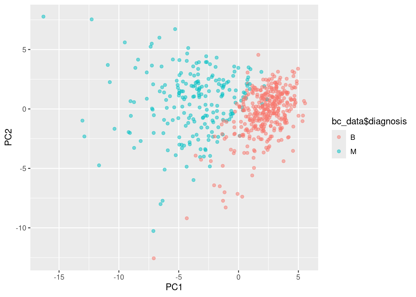
Teşhis bilgisi için her bileşeni ayrıca inceleyelim:
g_pc1 <- ggplot(pca_df, aes(x=PC1, fill=bc_data$diagnosis)) + geom_density(alpha=0.25)
g_pc2 <- ggplot(pca_df, aes(x=PC2, fill=bc_data$diagnosis)) + geom_density(alpha=0.25)
ggarrange(g_pc1, g_pc2, ncol=2, common.legend = T)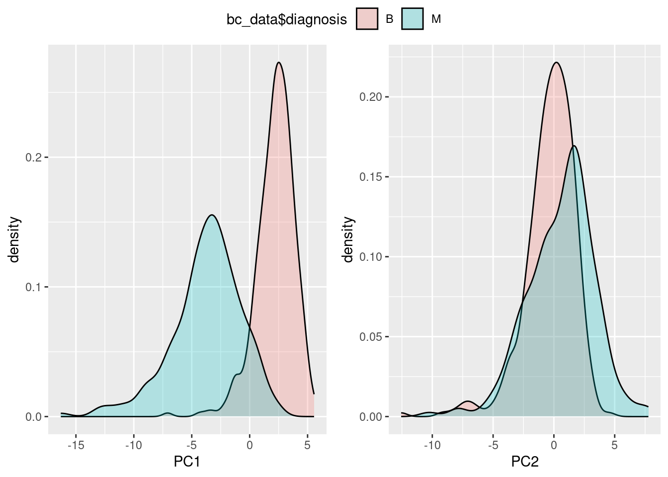
Modeli oluşturalım ve görüntüleyelim:
fitControl <- trainControl(method="cv", number = 5, preProcOptions = list(thresh = 0.99), classProbs = TRUE, summaryFunction = twoClassSummary)

model_nb <- train(diagnosis~., train_data, method="nb", metric="ROC", preProcess=c('center', 'scale'), trace=FALSE, trControl=fitControl)
Modeli test edelim ve inceleyelim (bunu aslında yukarıda da yaptık)
Predict <- predict(model_nb,newdata = test_data)
confusionMatrix(Predict, test_data$diagnosis)
Confusion Matrix and Statistics
Reference
Prediction B M
B 102 10
M 5 53
Accuracy : 0.9118
95% CI : (0.8586, 0.9498)
No Information Rate : 0.6294
P-Value [Acc > NIR] : <2e-16
Kappa : 0.8077
Mcnemar's Test P-Value : 0.3017
Sensitivity : 0.9533
Specificity : 0.8413
Pos Pred Value : 0.9107
Neg Pred Value : 0.9138
Prevalence : 0.6294
Detection Rate : 0.6000
Detection Prevalence : 0.6588
Balanced Accuracy : 0.8973
'Positive' Class : B
Her tahmin yürütücü değişkenin outcome/çıktı üzerindeki etkilerini kıyaslayalım:
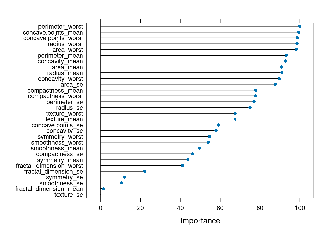
Yorum artık sizde, yukarıdaki grafiğe bakarak bir kişiye meme kanseri teşhisi konmasındaki en önemli etkenler hangileri olarak görünüyor?